An MRI scanner does not take a photograph. Nothing is shone through you and caught on a detector — there is no lens, no film, no X-ray. Instead the machine puts you in an enormous magnet, nudges the hydrogen nuclei in your body with a radio pulse, and then listens to the radio wave your own tissue emits as it settles back down. Stranger still, what it records is not a picture. It is the Fourier transform of one, measured line by line, and the image only appears after a computer transforms it back. This post builds the entire chain, starting from a single proton with nothing but a compass-needle analogy, and finishing at the reason a scan takes eight minutes and sounds like roadworks.
a spinning proton, a big magnet, and a radio pulse
1. Your body is full of tiny magnets
You are roughly 60 % water, and every water molecule carries two hydrogen atoms. The nucleus of an ordinary hydrogen atom is a single proton — and a proton has a property called spin, which for our purposes means one thing : it behaves like a minuscule bar magnet.
Left alone, those tiny magnets point in every direction at random, and their fields cancel out perfectly. Put them in a strong, uniform magnetic field $B_0$ and something small but crucial happens : very slightly more of them settle into the lower-energy orientation than the higher-energy one.
How slight ? This is worth computing, because the answer is genuinely surprising. The energy gap between the two orientations is $\Delta E = \gamma \hbar B_0$, and thermal jostling at body temperature is happy to knock spins between them. The Boltzmann factor gives the population imbalance :
\[\begin{equation} \frac{N_{\uparrow} - N_{\downarrow}}{N} \;\approx\; \frac{\Delta E}{2k_B T}. \label{eq:boltz} \end{equation}\]At $B_0 = 3$ tesla and $T = 310$ K, $\Delta E \approx 8.5 \times 10^{-26}$ J while $k_B T \approx 4.3 \times 10^{-21}$ J. The ratio is about one in a hundred thousand.
In plain words : of every 100,000 protons in your body, 99,999 cancel each other out exactly, and the entire multi-million-euro machine is built to detect the one that is left over.
It works only because there are so many protons. A single litre of water holds about $6.7 \times 10^{25}$ hydrogen nuclei, so even one part in $10^{5}$ leaves roughly $7 \times 10^{20}$ of them contributing — a number large enough to produce a measurable radio signal. Everything else in this post is about that vanishingly small surplus.
2. Spins do not just line up — they precess
Here is where the compass-needle picture needs upgrading. A compass needle in a field simply swings until it points along the field and stops. A proton does not, because it has angular momentum : it is spinning. A spinning object pushed sideways does not fall over, it precesses — it wheels around the direction of the push, exactly like a child’s spinning top wheeling slowly around the vertical while gravity pulls at it.
The rate of that wheeling is the single most important number in the subject.
Put numbers in and the whole design of the machine falls out. At 1.5 T the protons precess at 63.9 MHz ; at 3 T, at 127.7 MHz. Those are FM radio frequencies. That is why an MRI scanner is, underneath the plastic, a very precise radio transmitter and receiver wrapped around a magnet.
Read the Larmor equation once more, because Part III is nothing but its consequence : the precession frequency is proportional to the local field strength. If you can make the field vary across space in a controlled way, you make the frequency vary across space — and then frequency is position. That is the entire imaging trick, and it was Lauterbur’s insight in 1973 (Lauterbur, 1973).
3. Tipping the spins over
Right now the net magnetisation points straight along $B_0$, is perfectly steady, and induces nothing in any coil. To get a signal you must knock it sideways.
You do it by resonance. Transmit a radio pulse at exactly the Larmor frequency and the spins absorb it efficiently ; transmit at any other frequency and essentially nothing happens. It is the same phenomenon as pushing a child on a swing : tiny pushes timed to the swing’s own rhythm build up a large motion, while pushes at the wrong rhythm cancel themselves out. This selectivity is what the “resonance” in magnetic resonance imaging refers to 1, and it was demonstrated independently by Bloch (Bloch, 1946) and Purcell (Purcell et al., 1946) in 1946.
A pulse strong enough or long enough to knock the magnetisation fully into the transverse plane is called a 90° pulse. Now the magnetisation is spinning around in that plane at 63.9 MHz — and a rotating magnet next to a coil of wire induces a voltage in it, by plain Faraday induction.
In plain words : the scanner shouts at your protons in their own language, they answer back on the same frequency, and the antenna listens. Your body is the transmitter. The picture is built out of a radio signal that you emit.
two relaxation times, and the two knobs that exploit them
4. Relaxation : the two clocks
Switch the radio pulse off and the magnetisation returns to equilibrium. It does so by two independent processes running at once, and the fact that they are independent is the origin of all MRI contrast.
$T_2$ — transverse relaxation. The spins, each feeling slightly different fields from its neighbours, drift out of step with one another, so their vector sum shrinks even though no energy has left : $$ M_{xy}(t) = M_0\, e^{-t/T_2}. $$
In plain words : $T_1$ is how fast the spins settle back down, and it depends on how well the tissue can carry heat away at radio frequencies. $T_2$ is how fast they lose formation, like a marching band whose members drift out of step — nobody has stopped marching, but the group no longer moves as one. Losing formation is always at least as fast as settling down, so $T_2 \le T_1$ for every tissue.
The crucial point is that these are material properties, and different tissues have wildly different ones :
| tissue (approx., at 1.5 T) | $T_1$ | $T_2$ |
|---|---|---|
| fat | 260 ms | 80 ms |
| white matter | 780 ms | 90 ms |
| grey matter | 920 ms | 100 ms |
| muscle | 870 ms | 45 ms |
| cerebrospinal fluid | 4000 ms | 2000 ms |
Look at fat and cerebrospinal fluid : a factor of fifteen in $T_1$ and twenty-five in $T_2$. That enormous separation is why MRI distinguishes soft tissues that a CT scan renders as nearly identical grey mush — CT measures a single number, electron density, while MRI has at least three (proton density, $T_1$, $T_2$) and lets you choose which one to look at.
5. $T_2^{*}$, and the trick that recovers the signal
In practice the transverse signal dies much faster than $T_2$ suggests, because no magnet is perfectly uniform. A proton sitting where the field is a fraction stronger precesses a fraction faster and drifts ahead ; one in a weaker spot lags. The observed decay combines both effects :
\[\begin{equation} \frac{1}{T_2^{*}} = \underbrace{\frac{1}{T_2}}_{\text{genuine, random}} + \underbrace{\gamma \Delta B}_{\text{magnet imperfection}}. \label{eq:t2star} \end{equation}\]The second term is a nuisance — it tells you about your magnet, not the patient. But it has one redeeming property : it is deterministic. A proton in a slightly strong spot runs ahead by the same amount every time, and anything deterministic can be undone.
Hahn’s spin echo (Hahn, 1950) does exactly that, and the trick is genuinely beautiful. Wait a time $\tau$ while the spins fan out, then apply a 180° pulse that flips the whole fan over. The spins that had run ahead now find themselves behind by exactly as much — but they are still the fast ones, so after another interval $\tau$ they catch up precisely. Every spin arrives back in step at the same instant, and the signal reappears as an echo.
In plain words : runners on a track set off at different speeds and spread out. Blow a whistle and everyone turns around and runs back at their own unchanged pace. The fastest runner is furthest away but also covers ground fastest, so — provided nobody has changed speed — the whole field crosses the start line together.
What the echo cannot recover is the part where runners genuinely changed pace : the random, molecular-level dephasing. So the echo’s height is governed by true $T_2$, and the magnet’s imperfections have been cancelled out. This is why almost every clinical sequence is built on spin echoes.
6. Choosing what the image shows
You now have two timing knobs, and between them they decide which tissue property the picture displays.
- TR, the repetition time : how long you wait before exciting the same slice again. It controls how much $T_1$ recovery has happened.
- TE, the echo time : how long you wait before reading the echo. It controls how much $T_2$ decay has happened.
Three combinations cover most of clinical imaging, and each follows directly from the curves in figure 3 :
- Short TR, short TE → $T_1$-weighted. With a short TR, tissues that recover quickly (short $T_1$, like fat) are back near full magnetisation and give a strong signal, while slow ones (CSF) have barely recovered and stay dark. Short TE means $T_2$ has not had time to matter. Fat is bright, fluid is black. This is the anatomy view.
- Long TR, long TE → $T_2$-weighted. A long TR lets everything recover fully, erasing $T_1$ differences ; a long TE then lets the fast-decaying tissues fade while slow ones (CSF, and crucially oedema) remain. Fluid is brilliant white. This is the pathology view — inflammation, tumours and lesions almost all involve extra water.
- Long TR, short TE → proton-density weighted. Both differences suppressed, so brightness simply follows how much hydrogen is present.
gradients, k-space, and why it takes eight minutes
7. Making frequency mean position
So far every proton in the body sings the same note, and a single antenna hears them all mixed together. There is no spatial information at all. The fix is to deliberately ruin the uniformity of the field in a controlled, linear way, using extra coils called gradient coils :
\[\begin{equation} B(z) = B_0 + G_z\, z \quad\Longrightarrow\quad f(z) = \frac{\gamma}{2\pi}\big(B_0 + G_z z\big). \label{eq:grad} \end{equation}\]Now position is pitch. Three separate uses of this idea build the image.
Slice selection. Switch on $G_z$, then transmit an RF pulse containing only a narrow band of frequencies. Only the slab of tissue whose Larmor frequency falls inside that band is on resonance and gets tipped — everything above and below is untouched. The slice thickness follows directly :
\[\Delta z = \frac{\Delta f}{(\gamma/2\pi)\,G_z}.\]With a 1 kHz bandwidth and a 10 mT/m gradient, $\Delta z = 1000 / (42.58\times10^{6} \times 0.010) \approx 2.3$ mm. Want thinner slices ? Use a stronger gradient or a narrower band — and a narrower band means a longer pulse, which is the time-frequency uncertainty principle charging its usual fee.
Frequency encoding. Now switch on $G_x$ while listening. Every column of tissue sings at its own frequency, and the antenna picks up all of them superimposed. Separating them is precisely the prism problem : one Fourier transform of the recorded waveform and each column’s contribution falls into its own bin.
Phase encoding. That handles one axis ; the other needs a second trick. Before reading out, switch on $G_y$ briefly and then off. During that interval each row precesses at a different rate, so when the gradient stops, every row has been left with a different accumulated phase. Repeat the whole experiment with a different $G_y$ strength each time, and the row information is spread across repetitions.
8. k-space : the scanner measures a spectrum, not a picture
Now put those together and write down what the antenna actually receives. Every voxel contributes its own proton density $\rho(x,y)$, carrying whatever phase the gradients have given it. Defining the accumulated gradient area as
\[k_x(t) = \frac{\gamma}{2\pi}\int_0^t G_x(\tau)\,\mathrm{d}\tau, \qquad k_y(t) = \frac{\gamma}{2\pi}\int_0^t G_y(\tau)\,\mathrm{d}\tau,\]the received signal is
\[\begin{equation} S(k_x, k_y) = \iint \rho(x, y)\; e^{-2\pi i (k_x x + k_y y)}\;\mathrm{d}x\,\mathrm{d}y. \label{eq:kspace} \end{equation}\]Compare that with the definition of the Fourier transform and there is nothing left to prove :
The plane of $(k_x, k_y)$ is called k-space, and every scan is a plan for filling it in. In the standard sequence, each repetition applies one value of the phase-encoding gradient and reads out one horizontal line ; do that 256 times with 256 different $G_y$ values and you have a full grid.

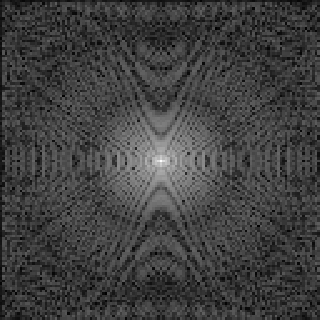
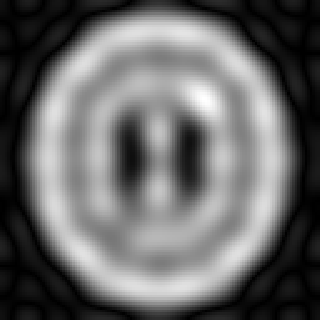
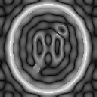
Figure 6 is the one to keep. The centre of k-space holds the low spatial frequencies : overall brightness and tissue contrast. The outskirts hold the high frequencies : edges and fine detail. Keep only the middle and you get a blurred image in which every tissue is still the right shade — which is why the centre lines are the ones that matter most for diagnosis. Keep only the outside and you get an outline drawing with no contrast at all.
9. Why it takes so long, and how they cheat
Look again at how k-space gets filled. One line per repetition, and each repetition costs a TR :
\[T_{\text{scan}} \;\approx\; \mathrm{TR} \times N_{\text{phase}} \times N_{\text{averages}}.\]With TR = 500 ms and 256 phase-encoding steps, that is 128 seconds for a single stack — and a full clinical protocol runs several sequences. This is the whole reason MRI is slow, and it is why the patient must lie still : the lines are collected minutes apart, so movement between them corrupts the entire image rather than one region of it. Every acceleration technique is an attack on that multiplication.
- Partial Fourier. The image is real-valued, and the transform of a real function is conjugate-symmetric — the bottom half of k-space is, in principle, the mirror of the top. Measure a little over half and infer the rest.
- Parallel imaging. Use several receive coils, each more sensitive to the part of the body nearest it. Skip every other k-space line ; the resulting image is aliased, exactly the folding described in the Fourier post — but because each coil sees a different weighted overlap, the fold can be algebraically undone. SENSE (Pruessmann et al., 1999) does this, and two to four times acceleration is routine.
- Compressed sensing. Sample k-space randomly rather than skipping regularly, so the artefacts are noise-like rather than coherent folds, then reconstruct by demanding that the image be sparse in some transform. Lustig and colleagues brought this to MRI in 2007 (Lustig et al., 2007) and it is now standard on clinical machines.
- Echo-planar imaging. Zig-zag through the whole of k-space after a single excitation (Mansfield, 1977). A complete image in under 100 ms, at the price of heavy distortion — which is an acceptable trade for functional and diffusion imaging, where you need speed far more than you need geometric fidelity.
10. What is actually in the room
It is worth knowing what the three components physically are, because two of them explain the experience of being scanned.
The main magnet is a superconducting solenoid — niobium-titanium wire bathed in liquid helium at about 4 K. Once the current is running it circulates with no resistance, so the field is never switched off, not overnight and not for maintenance. Removing it means deliberately boiling off the helium, a quench, which is expensive and takes days to undo. Every “MRI accident” story involving a chair or an oxygen cylinder flying across the room comes from this single fact.
The gradient coils are the noise. Each one carries tens of amperes and sits inside a 3 T field, so it feels an enormous Lorentz force ; switching it on and off hundreds of times a second makes the coil physically flex and bang against its mounting. The knocking you hear is the imaging happening, and it reaches 110 dB, which is why ear protection is not optional.
The RF coils transmit the pulse and receive the answer, often as an array of small coils placed close to the anatomy — the same array that makes parallel imaging possible.
There are two more limits that shape real protocols. SAR (specific absorption rate) caps how much RF energy may be deposited, because the pulses heat tissue. And switching gradients too fast induces currents in the patient’s own nerves, causing peripheral nerve stimulation — an involuntary twitch — which sets a hard ceiling on how quickly k-space can be traversed.
11. Beyond anatomy
The same hardware answers several quite different questions once you point the gradients at something other than position.
- Diffusion MRI. Add a pair of strong gradient pulses that cancel exactly for stationary spins but not for ones that moved in between. Signal loss then measures how far water molecules diffused. Since water in white matter diffuses preferentially along nerve fibres, mapping the directional dependence reconstructs the brain’s wiring.
- Functional MRI. Deoxygenated haemoglobin is paramagnetic and slightly distorts the local field, shortening $T_2^{*}$ ; oxygenated haemoglobin does not. Active brain regions receive more oxygenated blood than they consume, so their signal rises slightly. That is the BOLD effect (Ogawa et al., 1990). Worth stating plainly : fMRI measures blood oxygenation, not neural firing, and the inferential chain from one to the other is long — which is why the multiple-comparisons problem has bitten this field harder than most.
- Angiography and spectroscopy. Flowing blood can be made bright or dark by exploiting the fact that it leaves the slice between excitation and readout ; and the tiny chemical shifts in Larmor frequency between different molecules let you read out metabolite concentrations directly.
12. Conclusion
An MRI scanner is a chain of ideas, and each link is simple once the previous one is in place.
Your hydrogen nuclei are tiny magnets, and a huge field leaves a surplus of about one in a hundred thousand pointing the right way. That surplus precesses at a frequency set by the field strength, in the FM radio band. A pulse at exactly that frequency tips it over, and the tipped magnetisation induces a signal in an antenna — your body doing the transmitting. How that signal fades is governed by two independent tissue clocks, $T_1$ and $T_2$, and two timing knobs decide which of them the image displays.
Then the imaging trick : deliberately make the field vary across space, so that frequency and phase encode position. And with that, the thing the machine records stops being a picture and becomes a spectrum — equation $\eqref{eq:kspace}$ is the two-dimensional Fourier transform of the slice, sampled line by line. Everything about MRI follows from that. It is why scans take minutes rather than milliseconds, why motion ruins the whole image rather than a corner of it, why the middle of k-space matters more than the edges, and why the most effective ways to go faster are all arguments about how little of a Fourier transform you can get away with measuring.
The prism, again. Look at the world through frequency instead of space, and a problem that seemed to need a camera turns out to need an antenna and an inverse transform.
References
- Bloch, F. (1946). Nuclear Induction. Physical Review, 70(7–8), 460–474.
@article{Bloch1946, author = {Bloch, Felix}, title = {Nuclear Induction}, journal = {Physical Review}, volume = {70}, number = {7--8}, pages = {460--474}, year = {1946} } - Hahn, E. L. (1950). Spin Echoes. Physical Review, 80(4), 580–594.
@article{Hahn1950, author = {Hahn, Erwin L.}, title = {Spin Echoes}, journal = {Physical Review}, volume = {80}, number = {4}, pages = {580--594}, year = {1950} } - Lauterbur, P. C. (1973). Image Formation by Induced Local Interactions: Examples Employing Nuclear Magnetic Resonance. Nature, 242(5394), 190–191.
@article{Lauterbur1973, author = {Lauterbur, Paul C.}, title = {Image Formation by Induced Local Interactions: Examples Employing Nuclear Magnetic Resonance}, journal = {Nature}, volume = {242}, number = {5394}, pages = {190--191}, year = {1973} } - Lustig, M., Donoho, D., & Pauly, J. M. (2007). Sparse MRI: The Application of Compressed Sensing for Rapid MR Imaging. Magnetic Resonance in Medicine, 58(6), 1182–1195.
@article{Lustig2007, author = {Lustig, Michael and Donoho, David and Pauly, John M.}, title = {Sparse {MRI}: The Application of Compressed Sensing for Rapid {MR} Imaging}, journal = {Magnetic Resonance in Medicine}, volume = {58}, number = {6}, pages = {1182--1195}, year = {2007} } - Mansfield, P. (1977). Multi-Planar Image Formation Using NMR Spin Echoes. Journal of Physics C: Solid State Physics, 10(3), L55–L58.
@article{Mansfield1977, author = {Mansfield, Peter}, title = {Multi-Planar Image Formation Using {NMR} Spin Echoes}, journal = {Journal of Physics C: Solid State Physics}, volume = {10}, number = {3}, pages = {L55--L58}, year = {1977} } - Ogawa, S., Lee, T.-M., Kay, A. R., & Tank, D. W. (1990). Brain Magnetic Resonance Imaging with Contrast Dependent on Blood Oxygenation. Proceedings of the National Academy of Sciences, 87(24), 9868–9872.
@article{Ogawa1990, author = {Ogawa, Seiji and Lee, Tso-Ming and Kay, Alan R. and Tank, David W.}, title = {Brain Magnetic Resonance Imaging with Contrast Dependent on Blood Oxygenation}, journal = {Proceedings of the National Academy of Sciences}, volume = {87}, number = {24}, pages = {9868--9872}, year = {1990} } - Pruessmann, K. P., Weiger, M., Scheidegger, M. B., & Boesiger, P. (1999). SENSE: Sensitivity Encoding for Fast MRI. Magnetic Resonance in Medicine, 42(5), 952–962.
@article{Pruessmann1999, author = {Pruessmann, Klaas P. and Weiger, Markus and Scheidegger, Markus B. and Boesiger, Peter}, title = {{SENSE}: Sensitivity Encoding for Fast {MRI}}, journal = {Magnetic Resonance in Medicine}, volume = {42}, number = {5}, pages = {952--962}, year = {1999} } - Purcell, E. M., Torrey, H. C., & Pound, R. V. (1946). Resonance Absorption by Nuclear Magnetic Moments in a Solid. Physical Review, 69(1–2), 37–38.
@article{Purcell1946, author = {Purcell, Edward M. and Torrey, Henry C. and Pound, Robert V.}, title = {Resonance Absorption by Nuclear Magnetic Moments in a Solid}, journal = {Physical Review}, volume = {69}, number = {1--2}, pages = {37--38}, year = {1946} } - Twieg, D. B. (1983). The k-Trajectory Formulation of the NMR Imaging Process with Applications in Analysis and Synthesis of Imaging Methods. Medical Physics, 10(5), 610–621.
@article{Twieg1983,
  author = {Twieg, Donald B.},
  title = {The k-Trajectory Formulation of the {NMR} Imaging Process with Applications in Analysis and Synthesis of Imaging Methods},
  journal = {Medical Physics},
  volume = {10},
  number = {5},
  pages = {610--621},
  year = {1983}
}
-
The technique’s original name was nuclear magnetic resonance imaging, and it is still called NMR in chemistry and physics. The “nuclear” was quietly dropped for the medical version in the late 1970s, for the obvious public-relations reason — nothing about it is radioactive, and the word refers only to the fact that the signal comes from atomic nuclei rather than from electrons. ↩